An example of reading non-standard data using pandas and xarray#
It is very convenient when data is available in a format like netCDF, because it can be easily loaded using xarray.open_dataset, particularly when there is also sufficient metadata so the data can be identified and used correctly.
Sometimes data is only available in a non-standard form which takes some work to put into a convenient form like an xarray.Dataset. The purpose of this blog post is step through an example of the process of importing just such a dataset, transforming it into an easy to use xarray.Dataset, and then saving it as a netCDF formatted file for easy and convenient re-use.
Importing the Eastern Australia and New Zealand Drought Atlas (ANZDA) from NCEI, NOAA#
About the data: The data is a reconstruction of the Palmer drought sensitivity index across eastern Australia, and is the first Southern Hemisphere gridded drought atlas extending back to CE 1500.
The data is available from this NOAA website:
https://www.ncei.noaa.gov/access/paleo-search/study/20245
which explains the provenance of the data, has extensive meta-data in a number of formats, and a series of data files available for download
The data and grid information are stored in seprate files. Looking first at the grid, it is available in a text file (anzda-pdsi-xy.txt) as lat-lon pairs that correspond to each grid cell
The file is tab-delimited, and formatted into columns, the first column is longitude, the second latitude
168.25  -46.75  697     87      scPDSI.dat.
169.25  -46.25  699     88      scPDSI.dat.
169.75  -46.25  700     88      scPDSI.dat.
167.75  -45.75  696     89      scPDSI.dat.
168.25  -45.75  697     89      scPDSI.dat.
168.75  -45.75  698     89      scPDSI.dat.
169.25  -45.75  699     89      scPDSI.dat.
169.75  -45.75  700     89      scPDSI.dat.
As the data files are tab-separated columnar text files the pandas library is a good choice for reading in the data and manipulating it. pandas is specifically designed for manipulating tabular data, and much of the machinery of xarray is based on pandas, but extended to n-dimensions.
from datetime import datetime
import urllib

import numpy as np
import pandas as pd
import xarray as xr
Use the pandas.read_csv function to read the first two columns directly from the urlopen function, with the web address of the data file as a it’s argument, returning a pandas.Dataframe
Note that the delimiter is specifed to be be tab (\t), no header line is specified and the columns are assigned useful names.
url = "https://www.ncei.noaa.gov/pub/data/paleo/treering/reconstructions/australia/palmer2015pdsi/anzda-pdsi-xy.txt"
xy = pd.read_csv(urllib.request.urlopen(url),
                 delimiter='\t',
                 header = None,
                 names = ('lon', 'lat'),
                 usecols = [0, 1])
The head method is a useful way to get a small sample of the data to check it
xy.head()
| lon | lat | |
|---|---|---|
| 0 | 168.25 | -46.75 |
| 1 | 169.25 | -46.25 |
| 2 | 169.75 | -46.25 |
| 3 | 167.75 | -45.75 |
| 4 | 168.25 | -45.75 |
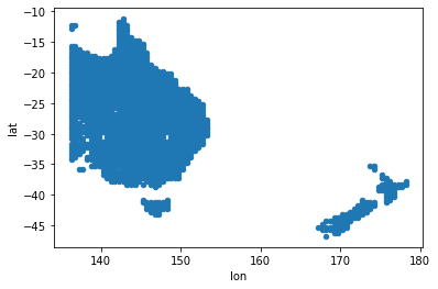
Plotting is also a great way to quickly check the data. Like xarray, pandas has a built in plot method that calls out to another library to do the plotting. In this case the default is matplotlib.
xy.plot(x='lon', y='lat', kind='scatter');
Now get the actual data: it is also tab-separated columnar ASCII format, according to the dataset README. That is, one reconstruction per column, with the grid cell number as the column header, and rows are by year with the first column the year index.
As before use the pandas.read_csv function to read the data in, specifying that the delimiter is a tab and that the first column should be treated as the row index. In this case the first line contains useful header information, so that is retained.
url = "https://www.ncei.noaa.gov/pub/data/paleo/treering/reconstructions/australia/palmer2015pdsi/anzda-recon.txt"
data = pd.read_csv(urllib.request.urlopen(url), delimiter='\t', index_col=0)
data
| 1 | 2 | 3 | 4 | 5 | 6 | 7 | 8 | 9 | 10 | ... | 1366 | 1367 | 1368 | 1369 | 1370 | 1371 | 1372 | 1373 | 1374 | 1375 | |
|---|---|---|---|---|---|---|---|---|---|---|---|---|---|---|---|---|---|---|---|---|---|
| Year | |||||||||||||||||||||
| 1500 | 0.047 | 0.192 | 0.694 | 0.617 | 1.331 | 0.758 | 1.105 | 0.320 | 0.487 | 0.919 | ... | 0.149 | -2.415 | -2.645 | -1.689 | -0.309 | -1.834 | -0.861 | 0.409 | 0.294 | -0.922 |
| 1501 | -1.992 | -1.599 | -1.086 | -1.904 | -2.338 | -1.585 | -1.907 | -2.004 | -1.522 | -1.424 | ... | 0.558 | -3.001 | -2.530 | -1.298 | -0.397 | 0.203 | -1.984 | 0.582 | 0.919 | -0.882 |
| 1502 | -0.551 | -0.491 | -0.333 | -0.901 | -0.550 | -1.249 | -1.408 | -0.623 | -0.296 | -0.840 | ... | -0.860 | -2.371 | -3.420 | -3.060 | -2.128 | -2.107 | -0.905 | -1.918 | -0.450 | -1.893 |
| 1503 | -2.560 | -2.793 | -1.539 | -2.449 | -2.696 | -2.232 | -2.962 | -2.576 | -1.995 | -0.980 | ... | 0.531 | -0.522 | 0.442 | 0.608 | -1.790 | 0.352 | -0.073 | -1.621 | 1.114 | -2.080 |
| 1504 | -1.729 | -1.835 | -1.514 | -1.830 | -1.867 | -1.225 | -1.918 | -2.063 | -1.577 | -0.832 | ... | -0.739 | -2.633 | -0.383 | -0.389 | -2.514 | -1.226 | -1.999 | -2.465 | -0.348 | -2.525 |
| ... | ... | ... | ... | ... | ... | ... | ... | ... | ... | ... | ... | ... | ... | ... | ... | ... | ... | ... | ... | ... | ... |
| 2008 | -1.058 | -0.663 | -0.271 | -1.061 | -1.050 | -0.613 | -0.840 | -0.549 | -0.103 | -0.461 | ... | 2.295 | 1.619 | -2.157 | -1.629 | 1.634 | 1.566 | 2.204 | 1.155 | 1.769 | 2.149 |
| 2009 | -0.072 | 0.554 | 0.662 | 0.923 | 1.133 | 0.621 | 0.410 | 0.438 | 1.037 | 0.895 | ... | 2.048 | 0.789 | -0.924 | -0.589 | 1.424 | 0.920 | 1.550 | 0.982 | 2.232 | 1.643 |
| 2010 | -0.488 | 0.077 | 0.295 | 0.006 | 1.873 | 0.237 | 0.083 | 0.114 | 0.400 | 0.299 | ... | 0.505 | -0.491 | 1.526 | 1.644 | -0.016 | -0.050 | 0.557 | -0.255 | 1.056 | 0.949 |
| 2011 | 0.015 | 0.510 | 1.889 | 0.489 | 1.893 | 0.644 | 0.613 | 1.871 | 1.744 | 0.935 | ... | 4.338 | 4.343 | 2.736 | 2.717 | 3.498 | 3.673 | 4.027 | 2.872 | 3.792 | 3.163 |
| 2012 | 0.218 | 0.490 | 0.519 | 0.506 | 0.766 | 0.614 | 0.503 | 0.391 | 0.344 | 1.219 | ... | 3.412 | 2.993 | 1.799 | 2.064 | 2.841 | 2.936 | 3.320 | 2.085 | 3.422 | 2.846 |
513 rows × 1375 columns
The data is stored as a matrix with associated time and location vectors, so we need to convert from a “wide” to “long” format using the melt method, with the result that there is a row for every unique combination of year and location.
Specifying ignore_index=False means it isn’t included in the value column, but is retained as an index. This method will create two new columns with the cell index in one, and the values from the table in other. The function has default names variable and value, but better to give them useful names: cellref and pdsi respectively.
data_long = data.melt(ignore_index=False, var_name = 'cellref', value_name='pdsi')
data_long
| cellref | pdsi | |
|---|---|---|
| Year | ||
| 1500 | 1 | 0.047 |
| 1501 | 1 | -1.992 |
| 1502 | 1 | -0.551 |
| 1503 | 1 | -2.560 |
| 1504 | 1 | -1.729 |
| ... | ... | ... |
| 2008 | 1375 | 2.149 |
| 2009 | 1375 | 1.643 |
| 2010 | 1375 | 0.949 |
| 2011 | 1375 | 3.163 |
| 2012 | 1375 | 2.846 |
705375 rows × 2 columns
Next is to add the lat and lon values for each cell index to the data table above. One way to achieve this is to add a cellref column to the xy table so it can be merged with data_long using the cellref variable as a key
xy['cellref'] = range(1, len(xy)+1, 1)
xy
| lon | lat | cellref | |
|---|---|---|---|
| 0 | 168.25 | -46.75 | 1 |
| 1 | 169.25 | -46.25 | 2 |
| 2 | 169.75 | -46.25 | 3 |
| 3 | 167.75 | -45.75 | 4 |
| 4 | 168.25 | -45.75 | 5 |
| ... | ... | ... | ... |
| 1370 | 142.75 | -12.25 | 1371 |
| 1371 | 143.25 | -12.25 | 1372 |
| 1372 | 142.25 | -11.75 | 1373 |
| 1373 | 142.75 | -11.75 | 1374 |
| 1374 | 142.75 | -11.25 | 1375 |
1375 rows × 3 columns
Now try merge
data_long.merge(xy, on='cellref')
---------------------------------------------------------------------------
ValueError                                Traceback (most recent call last)
Input In [8], in <cell line: 1>()
----> 1 data_long.merge(xy, on='cellref')

File /g/data/hh5/public/apps/miniconda3/envs/analysis3-22.01/lib/python3.9/site-packages/pandas/core/frame.py:9190, in DataFrame.merge(self, right, how, on, left_on, right_on, left_index, right_index, sort, suffixes, copy, indicator, validate)
   9171 @Substitution("")
   9172 @Appender(_merge_doc, indents=2)
   9173 def merge(
   (...)
   9186     validate: str | None = None,
   9187 ) -> DataFrame:
   9188     from pandas.core.reshape.merge import merge
-> 9190     return merge(
   9191         self,
   9192         right,
   9193         how=how,
   9194         on=on,
   9195         left_on=left_on,
   9196         right_on=right_on,
   9197         left_index=left_index,
   9198         right_index=right_index,
   9199         sort=sort,
   9200         suffixes=suffixes,
   9201         copy=copy,
   9202         indicator=indicator,
   9203         validate=validate,
   9204     )

File /g/data/hh5/public/apps/miniconda3/envs/analysis3-22.01/lib/python3.9/site-packages/pandas/core/reshape/merge.py:106, in merge(left, right, how, on, left_on, right_on, left_index, right_index, sort, suffixes, copy, indicator, validate)
     89 @Substitution("\nleft : DataFrame or named Series")
     90 @Appender(_merge_doc, indents=0)
     91 def merge(
   (...)
    104     validate: str | None = None,
    105 ) -> DataFrame:
--> 106     op = _MergeOperation(
    107         left,
    108         right,
    109         how=how,
    110         on=on,
    111         left_on=left_on,
    112         right_on=right_on,
    113         left_index=left_index,
    114         right_index=right_index,
    115         sort=sort,
    116         suffixes=suffixes,
    117         copy=copy,
    118         indicator=indicator,
    119         validate=validate,
    120     )
    121     return op.get_result()

File /g/data/hh5/public/apps/miniconda3/envs/analysis3-22.01/lib/python3.9/site-packages/pandas/core/reshape/merge.py:703, in _MergeOperation.__init__(self, left, right, how, on, left_on, right_on, axis, left_index, right_index, sort, suffixes, copy, indicator, validate)
    695 (
    696     self.left_join_keys,
    697     self.right_join_keys,
    698     self.join_names,
    699 ) = self._get_merge_keys()
    701 # validate the merge keys dtypes. We may need to coerce
    702 # to avoid incompatible dtypes
--> 703 self._maybe_coerce_merge_keys()
    705 # If argument passed to validate,
    706 # check if columns specified as unique
    707 # are in fact unique.
    708 if validate is not None:

File /g/data/hh5/public/apps/miniconda3/envs/analysis3-22.01/lib/python3.9/site-packages/pandas/core/reshape/merge.py:1256, in _MergeOperation._maybe_coerce_merge_keys(self)
   1250     # unless we are merging non-string-like with string-like
   1251     elif (
   1252         inferred_left in string_types and inferred_right not in string_types
   1253     ) or (
   1254         inferred_right in string_types and inferred_left not in string_types
   1255     ):
-> 1256         raise ValueError(msg)
   1258 # datetimelikes must match exactly
   1259 elif needs_i8_conversion(lk.dtype) and not needs_i8_conversion(rk.dtype):

ValueError: You are trying to merge on object and int64 columns. If you wish to proceed you should use pd.concat
The merge fails with an error message
You are trying to merge on object and int64 columns.
Inspecting the types (dtypes) of the two tables shows the issue, the cellref column in data_long has a type object
xy.dtypes
lon        float64
lat        float64
cellref      int64
dtype: object
data_long.dtypes
cellref     object
pdsi       float64
dtype: object
The solution is to replace the cellref column with the same data converted to a number, and try merging again.
data_long['cellref'] = pd.to_numeric(data_long['cellref'])
data_long
| cellref | pdsi | |
|---|---|---|
| Year | ||
| 1500 | 1 | 0.047 |
| 1501 | 1 | -1.992 |
| 1502 | 1 | -0.551 |
| 1503 | 1 | -2.560 |
| 1504 | 1 | -1.729 |
| ... | ... | ... |
| 2008 | 1375 | 2.149 |
| 2009 | 1375 | 1.643 |
| 2010 | 1375 | 0.949 |
| 2011 | 1375 | 3.163 |
| 2012 | 1375 | 2.846 |
705375 rows × 2 columns
Note that reset_index converts the Year index into a normal column, this is necessary to retain the Year as indices are discarded when a column is used as the value to merge with as is done here, i.e. on='cellref'
data_long = data_long.reset_index().merge(xy, on='cellref')
data_long
| Year | cellref | pdsi | lon | lat | |
|---|---|---|---|---|---|
| 0 | 1500 | 1 | 0.047 | 168.25 | -46.75 |
| 1 | 1501 | 1 | -1.992 | 168.25 | -46.75 |
| 2 | 1502 | 1 | -0.551 | 168.25 | -46.75 |
| 3 | 1503 | 1 | -2.560 | 168.25 | -46.75 |
| 4 | 1504 | 1 | -1.729 | 168.25 | -46.75 |
| ... | ... | ... | ... | ... | ... |
| 705370 | 2008 | 1375 | 2.149 | 142.75 | -11.25 |
| 705371 | 2009 | 1375 | 1.643 | 142.75 | -11.25 |
| 705372 | 2010 | 1375 | 0.949 | 142.75 | -11.25 |
| 705373 | 2011 | 1375 | 3.163 | 142.75 | -11.25 |
| 705374 | 2012 | 1375 | 2.846 | 142.75 | -11.25 |
705375 rows × 5 columns
The resulting dataframe has a value of pdsi for every year at every location, with an associated lat and lon value
Convert the dataframe to xarray#
Now the pandas dataframe can be converted to an xarray dataset, which is a well used standard for spatial data analysis. There is a handy function for this purpose, to_xarray.
Some commands are chained before to_xarray:
cellrefcolumn is dropped as it is no longer neededYearcolumn to renamed toyearkeep it tidy and case consistentset_indexcreates a multi-index
All the index variables created with set_index will automatically be converted to coordinates in the xarray object. The order of variables in set_index is important: longitude is set to be the fastest varying axis/index, which will result in plots being correctly oriented by default, with longitude on the horizontal axis.
ds = data_long.drop('cellref', axis=1).rename(columns={'Year': 'year'}).set_index(['year', 'lat', 'lon']).to_xarray()
ds
<xarray.Dataset>
Dimensions:  (year: 513, lat: 72, lon: 58)
Coordinates:
  * year     (year) int64 1500 1501 1502 1503 1504 ... 2008 2009 2010 2011 2012
  * lat      (lat) float64 -46.75 -46.25 -45.75 -45.25 ... -12.25 -11.75 -11.25
  * lon      (lon) float64 136.2 136.8 137.2 137.8 ... 176.8 177.2 177.8 178.2
Data variables:
pdsi (year, lat, lon) float64 nan nan nan nan nan ... nan nan nan nanPlot as a sanity check using the in-built plot method.
There appears to be a problem: data extended into the Tasman sea from both land masses.
ds.pdsi.isel(year=50).plot(size = 8);
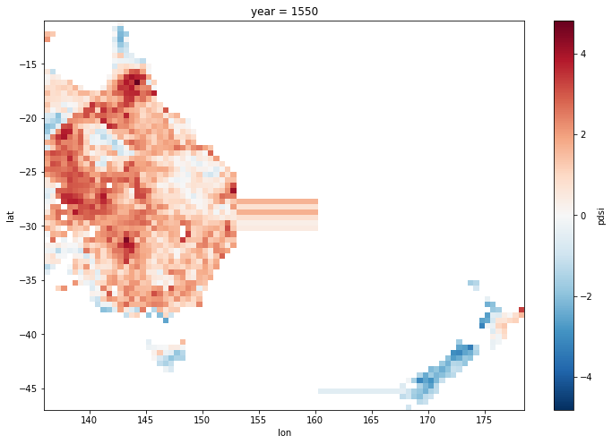
Looking at the difference between each longitude point and it’s neighbour shows the problem: there is difference of -14. at one point, so there is a gap in the coordinates in the Tasman Sea. This is because there are no data points with those longitudes in the original data set.
ds.coords['lon'] - ds.coords['lon'].shift({'lon':-1})
<xarray.DataArray 'lon' (lon: 58)>
array([ -0.5,  -0.5,  -0.5,  -0.5,  -0.5,  -0.5,  -0.5,  -0.5,  -0.5,
        -0.5,  -0.5,  -0.5,  -0.5,  -0.5,  -0.5,  -0.5,  -0.5,  -0.5,
        -0.5,  -0.5,  -0.5,  -0.5,  -0.5,  -0.5,  -0.5,  -0.5,  -0.5,
        -0.5,  -0.5,  -0.5,  -0.5,  -0.5,  -0.5,  -0.5, -14. ,  -0.5,
        -0.5,  -0.5,  -0.5,  -0.5,  -0.5,  -0.5,  -0.5,  -0.5,  -0.5,
        -0.5,  -0.5,  -0.5,  -0.5,  -0.5,  -0.5,  -0.5,  -0.5,  -0.5,
        -0.5,  -0.5,  -0.5,   nan])
Coordinates: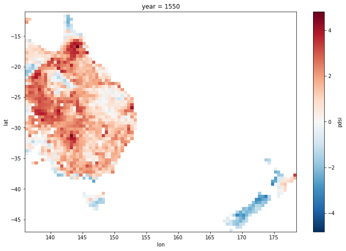
* lon (lon) float64 136.2 136.8 137.2 137.8 ... 176.8 177.2 177.8 178.2Fix this by creating a new longitude coordinate that spans the whole range with the same 0.5 degree spacing, and then replace the existing longitude coordinate using reindex
ds = ds.reindex(lon = xr.DataArray(np.arange(ds.lon.min(), ds.lon.max()+0.5, 0.5), dims=['lon']))
Now the same plot shows the correct behaviour, with no strange artefacts in the Tasman Sea
ds.pdsi.isel(year=50).plot(x='lon',y='lat', size = 8);
Save data for reuse#
First step is to add some meta-data. The website says:
Use Constraints:
Please cite original publication, online resource, dataset and publication DOIs (where available), and date accessed when using downloaded data. If there is no publication information, please cite investigator, title, online resource, and date accessed. The appearance of external links associated with a dataset does not constitute endorsement by the Department of Commerce/National Oceanic and Atmospheric Administration of external Web sites or the information, products or services contained therein. For other than authorized activities, the Department of Commerce/NOAA does not exercise any editorial control over the information you may find at these locations. These links are provided consistent with the stated purpose of this Department of Commerce/NOAA Web site.
Set the global (dataset level) attributes
ds.attrs = {
    "title": "Eastern Australia and New Zealand Drought Atlas (ANZDA)",
    "creator_name": "Palmer, J.G.; Cook, E.R.; Turney, C.S.M.; Allen, K.J.; Fenwick, P.; Cook, B.I.; O'Donnell, A.J.; Lough, J.M.; Grierson, P.F.; Baker, P.J.",
    "publisher": "National Centers for Environmental Information, NESDIS, NOAA, U.S. Department of Commerce",
    "references": "Jonathan G. Palmer, Edward R. Cook, Chris S.M. Turney, Kathy Allen, Pavla Fenwick, Benjamin I. Cook, Alison O'Donnell, Janice Lough, Pauline Grierson, Patrick Baker. 2015. Drought variability in the eastern Australia and New Zealand summer drought atlas (ANZDA, CE 1500-2012) modulated by the Interdecadal Pacific Oscillation. Environmental Research Letters, 10(12), 124002. doi:10.1088/1748-9326/10/12/124002",
    "keywords": "Palmer Drought Index Reconstruction, drought, paleoclimate",
    "date_created": "2016-06-06",
    "source": "https://www.ncei.noaa.gov/access/paleo-search/study/20245",
    "source_license": "Please cite original publication, online resource, dataset and publication DOIs (where available), and date accessed when using downloaded data. If there is no publication information, please cite investigator, title, online resource, and date accessed. The appearance of external links associated with a dataset does not constitute endorsement by the Department of Commerce/National Oceanic and Atmospheric Administration of external Web sites or the information, products or services contained therein. For other than authorized activities, the Department of Commerce/NOAA does not exercise any editorial control over the information you may find at these locations. These links are provided consistent with the stated purpose of this Department of Commerce/NOAA Web site.",
    "date_downloaded": datetime.today().strftime('%Y-%m-%d'),
    "geospatial_lat_min": -47.0,
    "geospatial_lat_max": -11.0,
    "geospatial_lon_min": 136.0,
    "geospatial_lon_max": 178.5,
    "time_coverage_start": "450 cal yr BP (1500 CE)",
    "time_coverage_end": "-62 cal yr BP (2012 CE)",
}
Next set variable level attributes
ds.pdsi.attrs = {
    "name": "Palmer drought severity index",
    "long_name": "Reconstructions of DJF Palmer drought severity index reconstruction series for 1375 Gridpoints",
    "units": "",
}
And coordinate attributes
ds.lon.attrs = {
    'name': 'longitude',
    'units': 'degrees_east',
}
ds.lat.attrs = {
    'name': 'latitude',
    'units': 'degrees_north',
}
Check the attributes have been specified correctly
ds
<xarray.Dataset>
Dimensions:  (lon: 85, year: 513, lat: 72)
Coordinates:
  * lon      (lon) float64 136.2 136.8 137.2 137.8 ... 176.8 177.2 177.8 178.2
  * year     (year) int64 1500 1501 1502 1503 1504 ... 2008 2009 2010 2011 2012
  * lat      (lat) float64 -46.75 -46.25 -45.75 -45.25 ... -12.25 -11.75 -11.25
Data variables:
    pdsi     (year, lat, lon) float64 nan nan nan nan nan ... nan nan nan nan
Attributes: (12/15)
    title:                Eastern Australia and New Zealand Drought Atlas (AN...
    creator_name:         Palmer, J.G.; Cook, E.R.; Turney, C.S.M.; Allen, K....
    publisher:            National Centers for Environmental Information, NES...
    references:           Jonathan G. Palmer, Edward R. Cook, Chris S.M. Turn...
    keywords:             Palmer Drought Index Reconstruction, drought, paleo...
    date_created:         2016-06-06
    ...                   ...
    geospatial_lat_min:   -47.0
    geospatial_lat_max:   -11.0
    geospatial_lon_min:   136.0
    geospatial_lon_max:   178.5
    time_coverage_start:  450 cal yr BP (1500 CE)
time_coverage_end: -62 cal yr BP (2012 CE)Save to a netcdf file
ds.to_netcdf("anzda_recon.nc", format = "NETCDF4")
Dump the file header to check it looks ok
!ncdump -h ~/anzda_recon.nc
netcdf anzda_recon {
dimensions:
	lon = 85 ;
	year = 513 ;
	lat = 72 ;
variables:
	double lon(lon) ;
		lon:_FillValue = NaN ;
		lon:name = "longitude" ;
		lon:units = "degrees_east" ;
	int64 year(year) ;
	double lat(lat) ;
		lat:_FillValue = NaN ;
		lat:name = "latitude" ;
		lat:units = "degrees_north" ;
	double pdsi(year, lat, lon) ;
		pdsi:_FillValue = NaN ;
		pdsi:name = "Palmer drought severity index" ;
		pdsi:long_name = "Reconstructions of DJF Palmer drought severity index reconstruction series for 1375 Gridpoints" ;
		pdsi:units = "" ;

// global attributes:
		:title = "Eastern Australia and New Zealand Drought Atlas (ANZDA)" ;
		:creator_name = "Palmer, J.G.; Cook, E.R.; Turney, C.S.M.; Allen, K.J.; Fenwick, P.; Cook, B.I.; O\'Donnell, A.J.; Lough, J.M.; Grierson, P.F.; Baker, P.J." ;
		:publisher = "National Centers for Environmental Information, NESDIS, NOAA, U.S. Department of Commerce" ;
		:references = "Jonathan G. Palmer, Edward R. Cook, Chris S.M. Turney, Kathy Allen, Pavla Fenwick, Benjamin I. Cook, Alison O\'Donnell, Janice Lough, Pauline Grierson, Patrick Baker. 2015. Drought variability in the eastern Australia and New Zealand summer drought atlas (ANZDA, CE 1500-2012) modulated by the Interdecadal Pacific Oscillation. Environmental Research Letters, 10(12), 124002. doi:10.1088/1748-9326/10/12/124002" ;
		:keywords = "Palmer Drought Index Reconstruction, drought, paleoclimate" ;
		:date_created = "2016-06-06" ;
		:source = "https://www.ncei.noaa.gov/access/paleo-search/study/20245" ;
		:source_license = "Please cite original publication, online resource, dataset and publication DOIs (where available), and date accessed when using downloaded data. If there is no publication information, please cite investigator, title, online resource, and date accessed. The appearance of external links associated with a dataset does not constitute endorsement by the Department of Commerce/National Oceanic and Atmospheric Administration of external Web sites or the information, products or services contained therein. For other than authorized activities, the Department of Commerce/NOAA does not exercise any editorial control over the information you may find at these locations. These links are provided consistent with the stated purpose of this Department of Commerce/NOAA Web site." ;
		:date_downloaded = "2022-03-18" ;
		:geospatial_lat_min = -47. ;
		:geospatial_lat_max = -11. ;
		:geospatial_lon_min = 136. ;
		:geospatial_lon_max = 178.5 ;
		:time_coverage_start = "450 cal yr BP (1500 CE)" ;
		:time_coverage_end = "-62 cal yr BP (2012 CE)" ;
}
Note: The year coordinate remains an integer, and has not been converted to a datetime format. It is possible to do so, but pandas does not support datetimes earlier than 1677-09-21 00:12:43.145225 and later than 2262-04-11 23:47:16.854775807. It is possible to convert to a cftime index, but it was not done for this example. This conversion would be necessary to use time based resampling or groupby.