Generating print-quality plots in R#
Some students have mentioned that they had generated plots with R and submitted them in their theses, but were requested to redo the plots at high resolution and to change the colour palette.
High Resolution#
If you use RStudio, you can click on the “Export” button and export your plots to a file in either PDF or PNG format. If you save it in PDF format, by default it is high resoultion. If, however, you wish to save it as a PNG bitmap, the default resolution will be 72 dpi (dots per inch), the standard screen resolution, far too low for high quality printing, which needs to be at least 300 dpi.
To see what I mean, let’s generate a plot as an example. We are will use a sample file recording maximum temperature available from the UK Met Office: https://www.metoffice.gov.uk/hadobs/hadghcnd/data/HadGHCND_1949-2011_TXx.nc.gz
We will now plot make a contour map displaying the average maximum temperature for the month of January:
library(ncdf4)
library(maps)

# load the heatwave data file
ncname <- "HadGHCND_1949-2011_TXx_1.nc"
ncin <- nc_open(ncname)

# extract lat, lon and January Tmax variables
lats <- rev(ncvar_get(ncin, "lat"))
lons <- ncvar_get(ncin, "lon")
janVals <- ncvar_get(ncin, "January")

# set up the matrix for the contour map
area <- matrix(0,nrow=dim(lons), ncol=dim(lats))
for (lat in 1:dim(lats)){
  for (lon in 1:dim(lons)){
    vals <- janVals[lon, dim(lats)+1-lat,]
    vals <- vals[!is.na(vals)]
    area[lon, lat] <- mean(vals)
  }
}

filled.contour(lons,lats,area,
                   xlim = range(lons), ylim = range(lats),
                   plot.axes = {axis(1);axis(2);
                     map('world',add=TRUE, wrap=c(-180,180), interior = FALSE)})
When saved in PNG format, you get this:
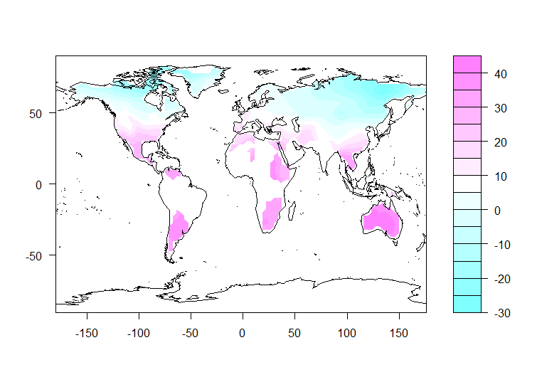 (You might not be able to see the low resolution so well here, but if you display the image on your browser you’ll definitely see it.)
The equivalent way to save to PNG file via the code is this:
png('heatMap.png', pointsize=10, width=700, height=480)
filled.contour(lons,lats,area,
                   xlim = range(lons), ylim = range(lats),
                   plot.axes = {axis(1);axis(2);
                     map('world',add=TRUE, wrap=c(-180,180), interior = FALSE)})
dev.off()
Increasing the resolution can be a bit tricky.
png('heatMap2.png', pointsize=10, width=700, height=480, res=300)
filled.contour(lons,lats,area,
                   xlim = range(lons), ylim = range(lats),
                   plot.axes = {axis(1);axis(2);
                     map('world',add=TRUE, wrap=c(-180,180), interior = FALSE)})
dev.off()
 Adding the
 res parameter fixes up the resolution, but it also rescales the axes and text. Therefore, you need to increase the height and the width.
png('heatmap3.png', pointsize=10, width=1400, height=960, res=300)
filled.contour(lons,lats,area,
               xlim = range(lons), ylim = range(lats),
               plot.axes = {axis(1);axis(2);
                 map('world',add=TRUE, wrap=c(-180,180), interior = FALSE)})
dev.off()
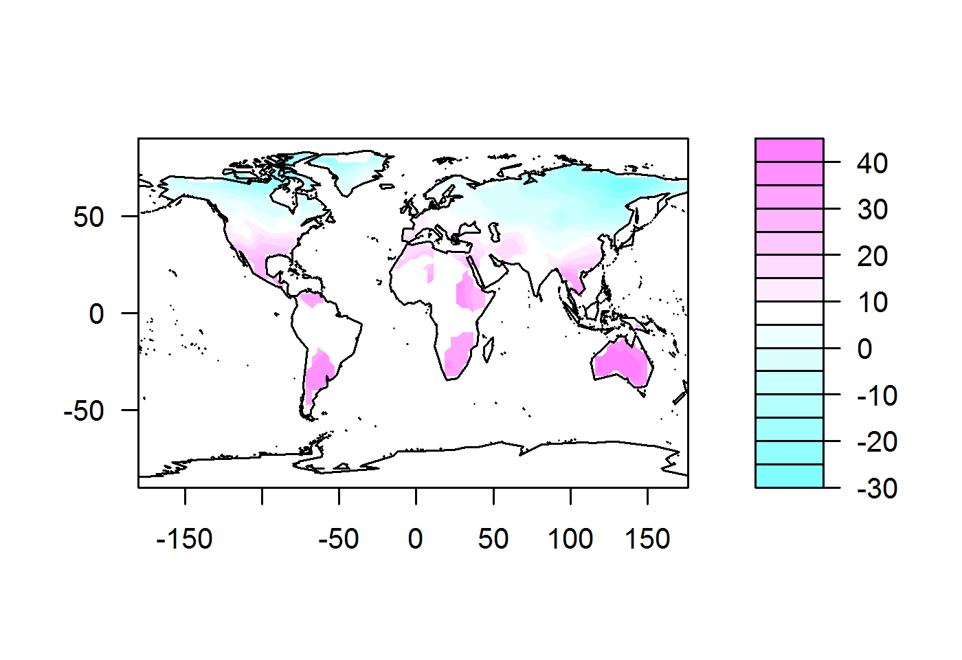
That’s better.
What if we want an even higher resolution, say 600dpi. So we change the first line to:
png('heatmap4.png', pointsize=10, width=2800, height=2000, res=600)
and run the plot again.
This time you might get the following error: Error in plot.new() : figure region too large.
What this means is that your figure doesn’t fit in the default device screen that R has set. What does that mean? Well, when you run a png() command, you are actually telling R to set up a PNG output device on which to display your plot. That device has certain default parameters, including dimensions and margin sizes. In this case, the plot you have specified doesn’t fit in the device’s spatial parameters.
You may be able to solve this problem by changing the device’s margin sizes. This may require a bit of fiddling to get them right. Margin sizes are measured in units of lines of text. (A plot has a specific text size.)
By adding a par(mar=...) command, my error went away.
png('heatmap4.png', pointsize=10, width=2800, height=2000, res=600)
par(mar=c(5, 4, 4, 2))
filled.contour(lons,lats,area,
               xlim = range(lons), ylim = range(lats),
               plot.axes = {axis(1);axis(2);
                 map('world',add=TRUE, wrap=c(-180,180), interior = FALSE)})
dev.off()
You may also get an error message saying that the margins are too big. That might indicate that:
You have to make them smaller, or
You haven’t set your plot dimensions to be sufficiently large, so there isn’t enough space to fit the margins.
Because this is so fiddly, it might just be easier to create a PDF file first, either with the Export function as discussed, or with the following script:
pdf('heatmap.pdf', pointsize=30, width=40, height=25)
filled.contour(lons,lats,area,
               xlim = range(lons), ylim = range(lats),
               plot.axes = {axis(1);axis(2);
                 map('world',add=TRUE, wrap=c(-180,180), interior = FALSE)})
dev.off()
Then you can convert it to the desired format. On the Mac, this can be done quite easily using Preview. Other tools that do this are ImageMagick or Adobe Acrobat. There are also a bunch of free online tools specifically for doing this kind of thing with PDFs, such as CombinePDF and SmallPDF.com.
(Note: I had to play a bit with the pointsize, width and height to get it right.)
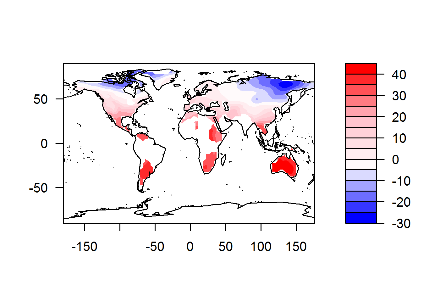
Changing the Colour Palette#
R’s default choice of colours is not to everyone’s taste and those submitting theses have been known to be asked to change the colour palette.
To set the colour palette for a plot, you just have to create a vector of colour names.
# create a vector with 15 shades ranging between the colours mentioned
colours = colorRampPalette(c("blue", "white", "pink", "red"))(15)
png('heatmap5.png', pointsize=10, width=1400, height=960, res=300, units="px")filled.contour(lons,lats,area, col=colours,
               xlim = range(lons), ylim = range(lats),
               plot.axes = {axis(1);axis(2);
                 map('world',add=TRUE, wrap=c(-180,180), interior = FALSE)})
dev.off()
Note that our colour palette has 15 shades. This needs to correspond to the number of colour levels in the plot. If you have too many shades, not all of them will be used; too few, and the colour palette will cycle (which is not very helpful).
For a full list of colour names in R, see here.
There are other colour tools you can use in R, such as RColorBrewer.
Happy plotting!