Visualisation in a Shiny App#
Supposing you have data you want to present in a way which will be intuitive to interpret. Perhaps you want to present it to colleagues, or perhaps as outreach to the public. What’s the best way to achieve that?
Effective visualisation is clearly the key to conveying your point. An interactive plot in a website could really make it happen. But how do you go about doing that?
Fortunately, there are a number of popular visualisation tools around designed to do this. In this post, we’re going to use Shiny, an R package that allows you to make interactive plot apps really easily. We’ll make an app which allows you to generate an interactive contour map of heatwave data.
Let’s Get Started#
Before you can create a Shiny app, you first have to install RStudio. (See https://www.rstudio.com/ for installation and other basics about using RStudio.)
Once you’ve done that, you’ll want to install some packages that we’ll be using in the Console window:
install.packages(c("shiny", "ncdf4", "maps", "colourpicker"))
(in some cases supporting packages may require compilation)
Create a new R script. We will start by importing the libraries our app will need:
## Basic Heatwave App ##

library(shiny)
library(ncdf4)
library(maps)
library(colourpicker)
The basic compnents of a Shiny app are the following 3 commands:
ui <- fluidPage()

server <- function(input, output) { }

#run/call the shiny app
shinyApp(ui, server)
The first command, ui <- fluidPage() tells Shiny what the UI - the user interface - will do. In other words, all your inputs which will be used for interactivity - such as slider inputs and select inputs - will be coded here.
The second command, server <- function(input, output) { } is the code for the server or the “back-end”. The server does the heavy lifting in terms of processing and will generate output which can be displayed on the screen.
The third command, shinyApp(ui, server) tells R to run the Shiny app.
Now run the app. (Some versions of RStudio have a Run App button. Otherwise, you might need to run it from a menu item: Code -> Run Region -> Run All.) It should bring up for you an empty browser window, indicating that your Shiny app works, but doesn’t yet do anything.
Providing Data For The App#
To correct this situation, let’s get our app to read in some data. Beforehand we downloaded some global heatwave data to our working directory which we will be using. For the purposes of this exercise, any global dataset should be fine. Above our ui <- fluidPage() command, let’s add in the following:
# load the heatwave data file
ncname <- "hw_ANN_CAM5-1-2degree_All-Hist_run001_1959-2012.nc"
ncin <- nc_open(ncname)
Now we’ll extract some basic variables from the files - lat, lon - with which we’ll calculate the dimensions for our contour map, as well as the names of the other variables in the data. We’ll set up the matrix of our contour map with these dimensions.
# extract lat, lon and variable names
lats <- ncvar_get(ncin, "lat")
lons <- ncvar_get(ncin, "lon")
varNames <- attributes(ncin$var)$names[4:23]

# set up the matrix for the contour map
area <- matrix(0,nrow=dim(lons), ncol=dim(lats))
Implementing the User Interface (UI)#
We’re now going to expand our ui <- fluidPage() to provide the controllers that will allow us to manipulate the plot. We will put our controllers in a sidebar panel on the left and there we will put 6 controllers:
A select input to select the variable from the data to plot.
A select input to select the statistic we wish to plot - mean, variance or standard deviation.
A slider input to choose the range of years of data to plot.
3 colour inputs to set the colours to use for the maximum, minimum and median values in the plot.
# implement the app's user interface
ui <- fluidPage(
  titlePanel("The Facts About Heatwaves"),

  # put the UI controllers in a sidebar
  sidebarLayout(

    sidebarPanel(

      # to select the variable
      selectInput("var", "Variable:", choices=varNames),

      # to select the statistic to apply
      selectInput("stat", "Statistic:",
                  choices=c("Mean", "Variance", "Standard Deviation")),

      # a slider to select the date range
      sliderInput("dateRange", "Date Range", min=1959, max=2012,
                  value=c(1959,2012), dragRange = TRUE, sep=""),

      # a slider to select the range of z values to include in the plot
      sliderInput("dataRange", "Data Range", min=-50, max=100,
                  value=c(-50,100), dragRange = TRUE, sep=""),

      # to select the colours you want for the max, min and median values
      colourInput("colMax", "Maximum Colour", "Red", showColour = "background"),
      colourInput("colMid", "Median Colour", "White", showColour = "background"),
      colourInput("colMin", "Minimum Colour", "Blue", showColour = "background")
    ),

    # The plot itself will display in the main panel, to the right of the side bar:
    mainPanel(
      plotOutput(outputId = "contourMap")
    )
  )
)
Let’s leave shinyApp(ui, server) at the bottom. If you run it now (i.e. click Run App), you should see the controllers in the side panel, with a space to the right where our plot will go. Now to implement the plot…
Implementing the Server Code#
We will now replace our server <- function(input, output) { } with server code that does something.
server <- function(input, output) {

  # Here is the code for the contour map that will be displayed in the main panel
  # renderPlot() creates a reactive plot, i.e. one that will change interactively with our controllers
  output$contourMap <- renderPlot( {

    # Use the value from the "stat" input
    calc <- input$stat

    # Set "fn" to the appropriate function call for that statistic - mean(), var() or sd()
    if (calc == "Mean")
      fn <- mean
    else if (calc == "Variance")
      fn <- var
    else
      fn <- sd

    # input$var is the selected variable to use. We will use the values of that variable from the file.
    varValues <- ncvar_get(ncin, input$var)

    # input$dateRange is the year range selected by the slider input
    dateRange = input$dateRange
    indexRange <- dateRange - 1958

    # go to every lat/lon point, take the variable's values over the entire time range,
    # apply the selected function on it and store it in the contour map's matrix
    for (lat in 1:dim(lats)){
      for (lon in 1:dim(lons)){
        vals <- varValues[lon, lat, indexRange[1]:indexRange[2]]

        # remove Na values
        vals <- vals[!is.na(vals)]
        area[lon, lat] <- fn(vals)
      }
    }

    # Create a palette with the 3 selected colours to use in the contour map
    colours = colorRampPalette(c(input$colMin, input$colMid, input$colMax))(24)

    # display the contour map with lat/lon axes and a world map
    filled.contour(lons,lats,area, col=colours, zlim =input$dataRange,
                   xlim = range(lons), ylim = range(lats),
                   plot.axes = {axis(1);axis(2);
                     map('world',add=TRUE, wrap=c(0,360), interior = FALSE)}
    )
  })
}
We can leave our shinyApp(ui, server) command as is.
And that’s it!
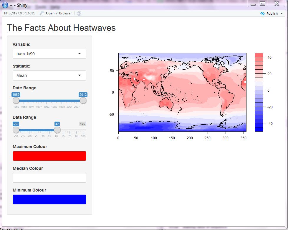
Now run the app and check it out. You should get something that looks like this (after adjusting the “Data Range” slider as shown):
If you want your app to be accessible on the internet, you’ll need to find somewhere to host your application (e.g. Nectar) and use Shiny Server to run it. To see an example of how that’s done, read this great tutorial.