Python Plotting Basics#
Let’s take a look at some basic plotting with Python
If you’d like to follow along, connect to VDI then in a terminal run:
module use /g/data3/hh5/public/modules
module load conda/analysis3
jupyter notebook
This will start up a Jupyter Notebook on VDI, which is the same tool that this post is written in. Jupyter lets us work interactively with python and easily share code and plots.
# This is a python command
print("Hello world!")

# the output appears below
Hello world!
Sample data#
To start out, let’s get some sample data to work with. NCI has a data store with all of the Australian CMIP5 data. You can find this on NCI’s Data Catlogue
I like to use a library called Xarray to work with netCDF datasets. Let’s grab the monthly surface temperature from the ACCESS1-0 AMIP run and load it in
import xarray

datapath = "http://dapds00.nci.org.au/thredds/dodsC/rr3/CMIP5/output1/CSIRO-BOM/ACCESS1-0/amip/mon/atmos/Amon/r1i1p1/latest/tas/tas_Amon_ACCESS1-0_amip_r1i1p1_197901-200812.nc"
data = xarray.open_dataset(datapath)
I’m accessing the data remotely here using what’s called a THREDDS URL. You could just as easily use the /g/data filepath if you’re running on VDI.
To see what’s in the file we can just print it. This shows the dimensions, variables and metadata in the file:
print(data)
<xarray.Dataset>
Dimensions:    (bnds: 2, lat: 145, lon: 192, time: 360)
Coordinates:
  * time       (time) datetime64[ns] 1979-01-16T12:00:00 1979-02-15 ...
  * lat        (lat) float64 -90.0 -88.75 -87.5 -86.25 -85.0 -83.75 -82.5 ...
  * lon        (lon) float64 0.0 1.875 3.75 5.625 7.5 9.375 11.25 13.12 15.0 ...
    height     float64 ...
Dimensions without coordinates: bnds
Data variables:
    time_bnds  (time, bnds) float64 ...
    lat_bnds   (lat, bnds) float64 ...
    lon_bnds   (lon, bnds) float64 ...
    tas        (time, lat, lon) float32 ...
Attributes:
    institution:                     CSIRO (Commonwealth Scientific and Indus...
    institute_id:                    CSIRO-BOM
    experiment_id:                   amip
    source:                          ACCESS1-0 2011. Atmosphere: AGCM v1.0 (N...
    model_id:                        ACCESS1-0
    forcing:                         GHG, Oz, SA, Sl, Vl, BC, OC, (GHG = CO2,...
    parent_experiment_id:            N/A
    parent_experiment_rip:           r1i1p1
    branch_time:                     0.0
    contact:                         The ACCESS wiki: http://wiki.csiro.au/co...
    history:                         CMIP5 compliant file produced from raw A...
    references:                      See http://wiki.csiro.au/confluence/disp...
    initialization_method:           1
    physics_version:                 1
    tracking_id:                     7cfe11fc-5b1c-457d-812b-e95f45e7def4
    version_number:                  v20120115
    product:                         output
    experiment:                      AMIP
    frequency:                       mon
    creation_date:                   2012-02-17T05:21:53Z
    Conventions:                     CF-1.4
    project_id:                      CMIP5
    table_id:                        Table Amon (01 February 2012) 01388cb450...
    title:                           ACCESS1-0 model output prepared for CMIP...
    parent_experiment:               N/A
    modeling_realm:                  atmos
    realization:                     1
    cmor_version:                    2.8.0
    DODS_EXTRA.Unlimited_Dimension:  time
Accessing variables#
Variables are accessed using dot syntax. Just like the full dataset we can print individual variables to see their metadata:
surface_temp = data.tas
print(surface_temp)
<xarray.DataArray 'tas' (time: 360, lat: 145, lon: 192)>
[10022400 values with dtype=float32]
Coordinates:
  * time     (time) datetime64[ns] 1979-01-16T12:00:00 1979-02-15 ...
  * lat      (lat) float64 -90.0 -88.75 -87.5 -86.25 -85.0 -83.75 -82.5 ...
  * lon      (lon) float64 0.0 1.875 3.75 5.625 7.5 9.375 11.25 13.12 15.0 ...
    height   float64 ...
Attributes:
    standard_name:     air_temperature
    long_name:         Near-Surface Air Temperature
    units:             K
    cell_methods:      time: mean
    cell_measures:     area: areacella
    history:           2012-02-17T05:21:51Z altered by CMOR: Treated scalar d...
    associated_files:  baseURL: http://cmip-pcmdi.llnl.gov/CMIP5/dataLocation...
Selecting data#
Before we can make a plot we first need to reduce the 3D data to 2D. One of the nice things about Xarray is that you can select data by a coordinate value, rather than manualy working out an index:
surface_temp_slice = surface_temp.sel(time = '1984-03')
print(surface_temp_slice.time)
<xarray.DataArray 'time' (time: 1)>
array(['1984-03-16T12:00:00.000000000'], dtype='datetime64[ns]')
Coordinates:
  * time     (time) datetime64[ns] 1984-03-16T12:00:00
    height   float64 ...
Attributes:
    bounds:         time_bnds
    axis:           T
    long_name:      time
    standard_name:  time
Plotting#
Now that we’ve selected our data we can get plotting
The notebook requires a special %matplotlib inline command to show plots, which isn’t needed if you’re writing a script.
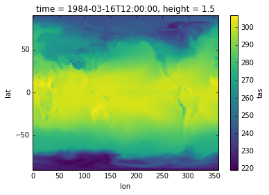
To make a quick plot we can just call .plot() on a 2d variable:
%matplotlib inline
import matplotlib.pyplot as plt

surface_temp_slice.plot()
plt.show()